Quarto Examples

This post demonstrates some basic functionalities of Quarto

Quarto Examples

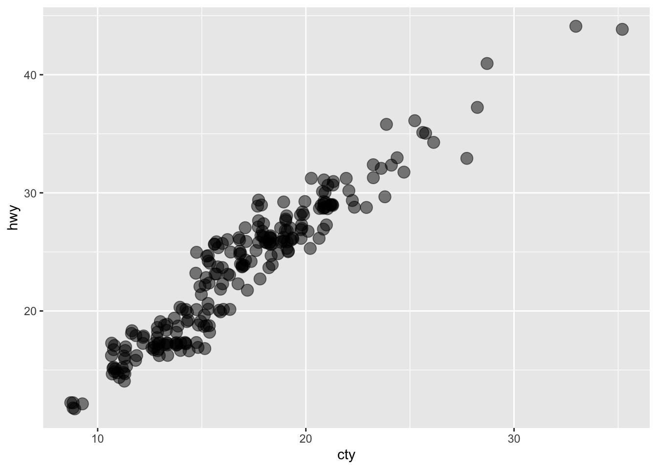
This post is mostly here for my education and to showcase Quarto’s capabilities. I snaged it from someone’s github project, so feel free to grab it from my repo as well. The idea is to have this as the first post to remind me how to do things in Quarto. The main parts of the this post which interests me are the latex, graphing, and code organization. Feel free to look through and let me know if there are any other Quarto featurs you would like to see added.

Section One

Lorem ipsum dolor sit amet, consectetur adipiscing elit. Nam suscipit est nec dui eleifend, at dictum elit ullamcorper. Aliquam feugiat dictum bibendum. Praesent fermentum laoreet quam, cursus volutpat odio dapibus in. Fusce luctus porttitor vehicula. Donec ac tortor nisi. Donec at lectus tortor. Morbi tempor, nibh non euismod viverra, metus arcu aliquet elit, sed fringilla urna leo vel purus.

Code

This is inline code plus a small code chunk.

library(tidyverse)

ggplot(mpg) +
  geom_jitter(aes(cty, hwy), size = 4, alpha = 0.5) 

Tabsets

The downloaded binary packages are in
    /var/folders/1w/2jhcvr5j3ks70z14vzn99pb40000gn/T//RtmptVyMtI/downloaded_packages

Transforming OLS estimates

install.packages("thematic", repos = "http://cran.us.r-project.org")
## 
## The downloaded binary packages are in
##  /var/folders/1w/2jhcvr5j3ks70z14vzn99pb40000gn/T//RtmptVyMtI/downloaded_packages


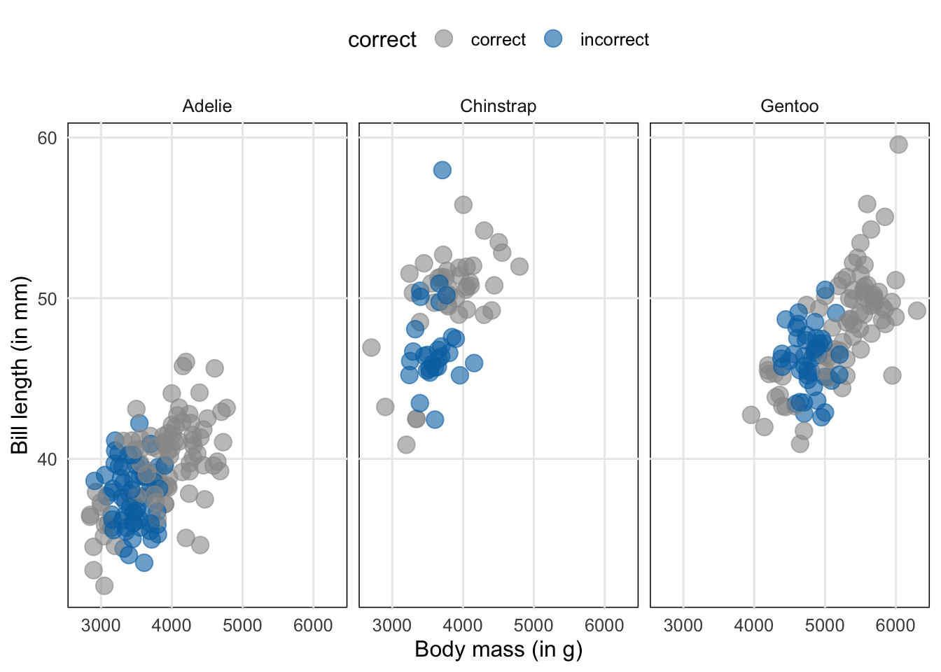
#| code-fold: true
preds_lm %>% 
  ggplot(aes(body_mass_g, bill_length_mm, col = correct)) +
  geom_jitter(size = 4, alpha = 0.6) +
  facet_wrap(vars(species)) +
  scale_color_manual(values = c('grey60', thematic::okabe_ito(3)[3])) +
  scale_x_continuous(breaks = seq(3000, 6000, 1000)) +
  theme_minimal(base_size = 12) +
  theme(
    legend.position = 'top', 
    panel.background = element_rect(color = 'black'),
    panel.grid.minor = element_blank()
  ) +
  labs(
    x = 'Body mass (in g)',
    y = 'Bill length (in mm)'
  )

Maximizing likelihood

Code

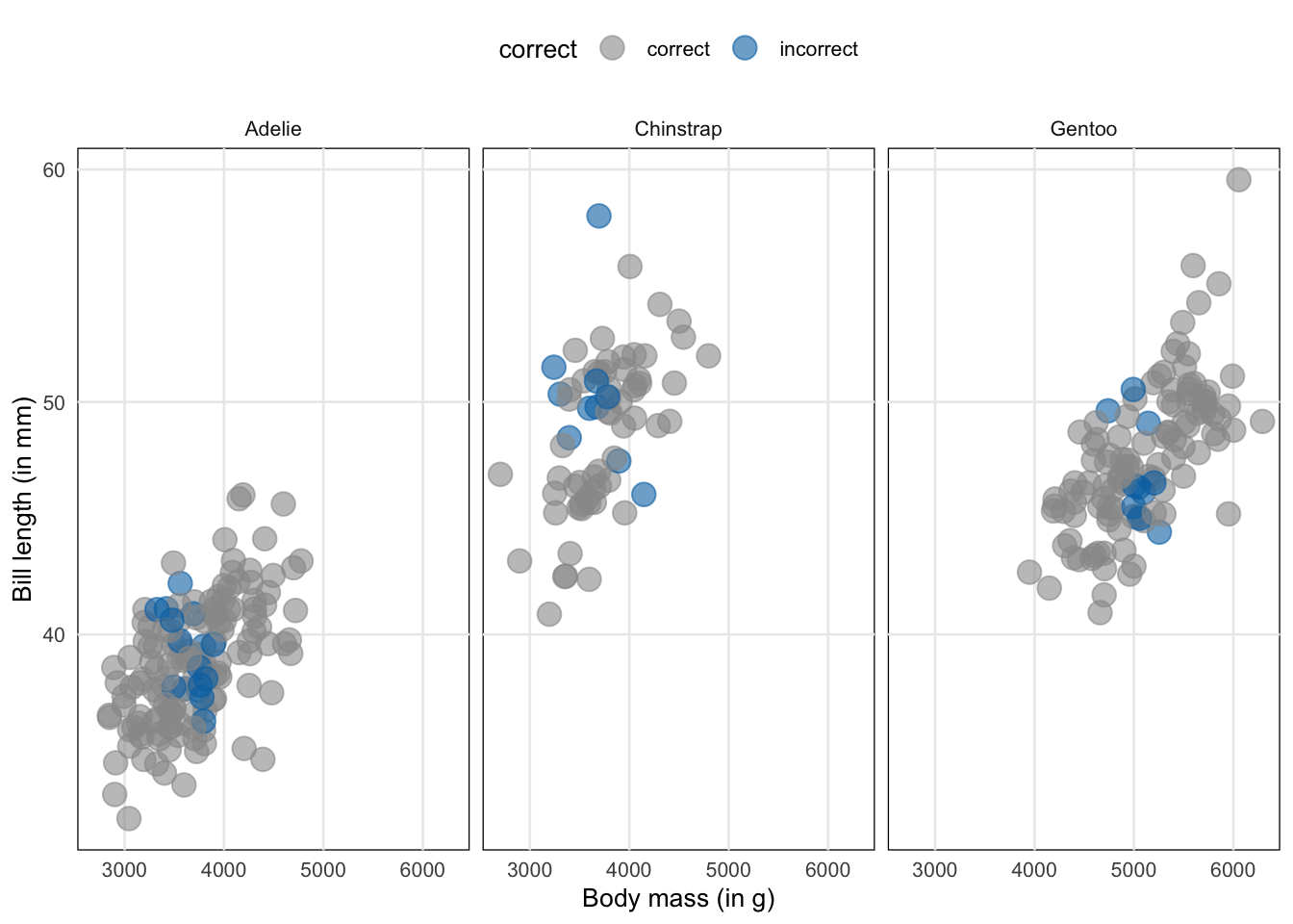
glm.mod <- glm(sex ~ body_mass_g + bill_length_mm + species, family = binomial, data = dat)

preds <- dat %>% 
  mutate(
    prob.fit = glm.mod$fitted.values,
    prediction = if_else(prob.fit > 0.5, 'male', 'female'),
    correct = if_else(sex == prediction, 'correct', 'incorrect')
  )


preds %>% 
  ggplot(aes(body_mass_g, bill_length_mm, col = correct)) +
  geom_jitter(size = 4, alpha = 0.6) +
  facet_wrap(vars(species)) +
  scale_x_continuous(breaks = seq(3000, 6000, 1000)) +
  scale_color_manual(values = c('grey60', thematic::okabe_ito(3)[3])) +
  theme_minimal(base_size = 10) +
  theme(
    legend.position = 'top', 
    panel.background = element_rect(color = 'black'),
    panel.grid.minor = element_blank()
  ) +
  labs(
    x = 'Body mass (in g)',
    y = 'Bill length (in mm)'
  )

Latex example

\[ \int_0^1 f(x) \ dx \]

Two Code Columns

geom_density(
  mapping = NULL,
  data = NULL,
  stat = "density",
  position = "identity",
  ...,
  na.rm = FALSE,
  orientation = NA,
  show.legend = NA,
  inherit.aes = TRUE,
  outline.type = "upper"
)

stat_density(
  mapping = NULL,
  data = NULL,
  geom = "area",
  position = "stack",
  ...,
  bw = "nrd0",
  adjust = 1,
  kernel = "gaussian",
  n = 512,
  trim = FALSE,
  na.rm = FALSE,
  orientation = NA,
  show.legend = NA,
  inherit.aes = TRUE
)

Margin captions

install.packages("gapminder", repos = "http://cran.us.r-project.org")
## 
## The downloaded binary packages are in
##  /var/folders/1w/2jhcvr5j3ks70z14vzn99pb40000gn/T//RtmptVyMtI/downloaded_packages

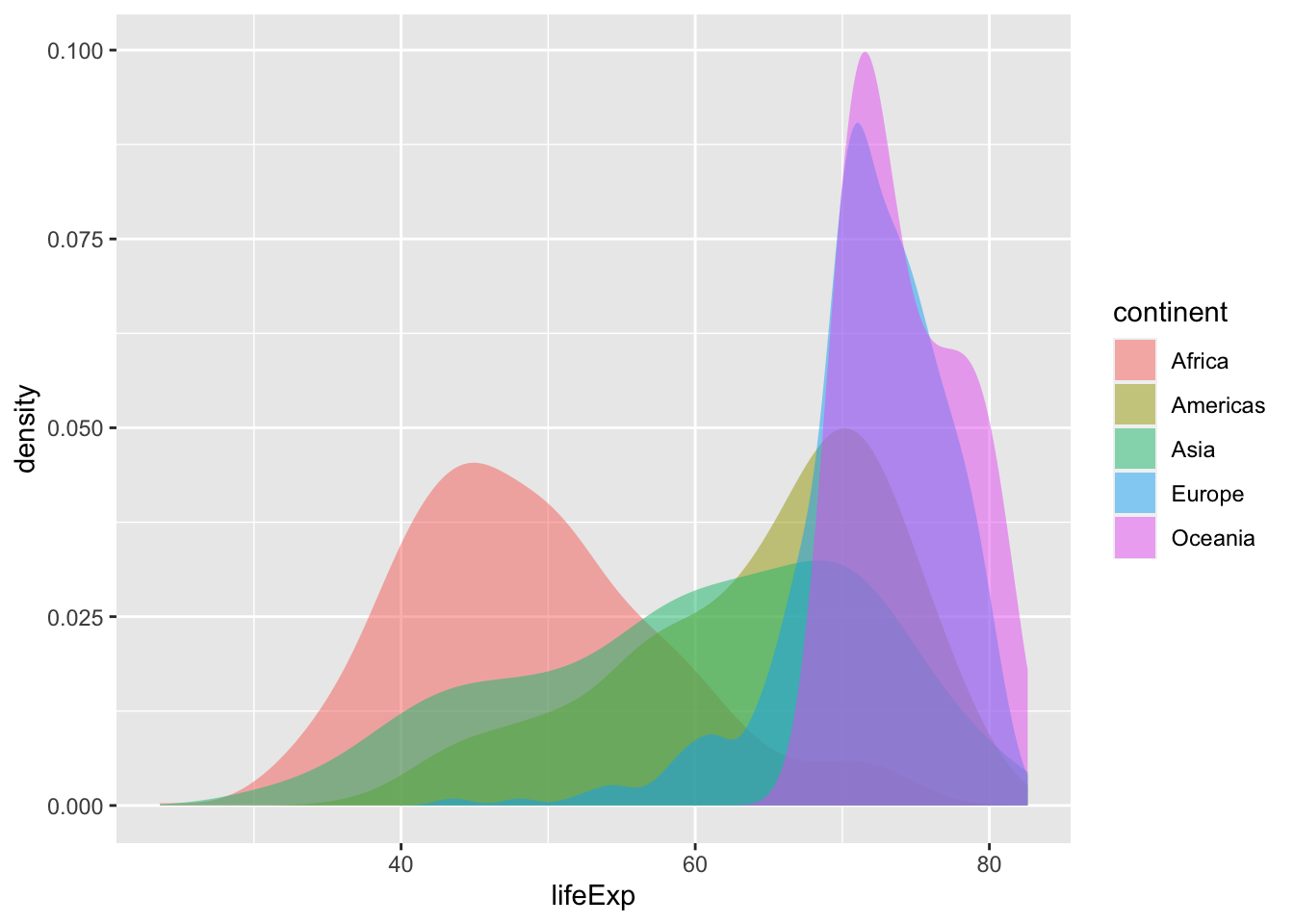
#| fig-cap: "Bla bla bla. This is a caption in the margin. Super cool isn't it?"
#| fig-cap-location: margin
ggplot(data = gapminder::gapminder, mapping = aes(x = lifeExp, fill = continent)) +
  stat_density(position = "identity", alpha = 0.5)